VAEs: When Neural Networks Learned Uncertainty

1.Introduction¶

On my journey to understand deep learning and regularization models, it only felt natural to explore Variational Autoencoders after working on Nonlinear PCA.Click here to learn more.
Variational Autoencoders are a form of Autoencoders which use probabilistic aproach on learning data and use a continous latent space.
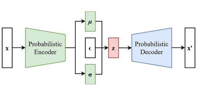
Structurally, a VAE looks almost identical to a standard Autoencoder. We still have:
Encoder --> Latent space --> Decoder
But conceptually, the difference is huge.

A regular Autoencoder is deterministic. Given a data point 𝑥 it determines a unique latent representation 𝑧 for that input. The mapping is fixed, so the same input will always produce the same latent vector.

In contrast, a Variational Autoencoder is probabilistic. Given a data point 𝑥, it determines a distribution over the latent space that is most likely to represent the data. Instead of committing to a single latent vector, it models a range of plausible representations from which z can be sampled and chooses from there accordingly

2.Defining the terms¶

Before we getting into the nuance of the math, lets define some terms which we will se throughout this blog

let's take:
- x as datapoint in the data
- z as variable from the latent space

note: all p() terms indiacte probablities

2.1 p(z)
This is called the prior. It represents our initial assumption of how the latent space is distributed, before observing any data.
It encodes what we belive the latent space to look like indpendent of any particular input. It is a structural assumption that keeps the model well-behaved.

2.2 p(x/z)
This represents the probablity of seeing a given data point x for a specifc variable z in the latent space.
In practice, the decoder tries to reconstruct x from z, and this probabilty tells us how accurate the reconstruction is

2.3 p(z/x)
This represents the true posterior . It shows, for a given data point x, what latent representation could have generated it
This is the quantity we idealy want to compute, but in practice it is very complicated to do that.

2.3.1 p(x) and its Intractablility
$$
[
p(x) = \int p(x \mid z)\, p(z)\, dz
]
$$
This expression gives the marginal likelihood of a data point or
It tells us how likely the model thinks the observed data is, after considering all possible latent variables that could have generated it.

However, this integral is intractable. an Intractable integral is on where there is no closed form solution once p(x/z) is modeled by a neural network, and evaluating it exactly would require integrating over infinitely many possible latent variables.
$$
[
p(z \mid x) = \frac{p(x \mid z)\, p(z)}{p(x)}
]
$$
since p(z/x) depends on p(x), we can not compute it.

so what do we do?

2.4.q(z/x)
This is the variational aproximation. Since we cant compute p(z/x) we introduce an aproximation
p(z/x) ~ q(z/x)
this is modeled by encoder, q(z/x) is formed after training a neural network to learn a distribution that is close to p(z/x)

2.5 Log Likelihood¶

Before getting into the next steps, let us pause and understand what we are actually trying to optimize.

At the end of the day, we want our model to explain the data well. For a single data point x, this is measured by the probability p(x). The higher this value, the better our model explains that data point.

For an entire dataset
$$[( {x^{(i)}}_{i=1}^{N} )],$$
we aim to maximize the joint likelihood,as in we want all data points likey under our model, so we maximize:

$$
[
\prod_{i=1}^{N} p(x^{(i)})
]$$
This product can become extremely small and difficult to work with, so instead we take the logarithm.
This turns the product into a sum:
$$
[
\log \left( \prod_{i=1}^{N} p(x^{(i)}) \right)
=
\sum_{i=1}^{N} \log p(x^{(i)})
]$$

This quantity is called the log likelihood.

We use the logarithm for two main reasons:

• It converts products into sums, making optimization easier.
• It improves numerical stability when dealing with very small probabilities.

Thus, in a Variational Autoencoder, our goal is to maximize:
$$
[
\log p(x)
]$$

3. ELBO¶

ELBO stands for Evidence Lower Bound.

To understand it, remember our real goal: we want to maximize the log likelihood
log(p(x)) which measures how well our model explains the data.

since we know that p(x) is not solvable. So we instead use a lowerboud on log(p(x)) rather than maximizing it.
Mathematically we can say,
$$
[
\log p(x) \ge \mathcal{L}_{\text{ELBO}}(x)
]$$
so, we can say that the ELBO is a function that is always less than or equal to log(p(x))
since ELBO is a lower bound on log(p(x)), then maximizing ELBO pushes the true log likelihood upward as well.

After simplifying, the equation for ELBO comes out as:

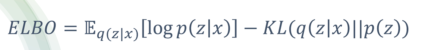
3.1 Expectation Function¶

Over here you see ,the RHS is made from 2 terms, one of them is the
$$
\mathbb{E}_{q(z|x)}[\log(p(x/z))]
$$
This is called the Expectaion Function. It can be understood as a weighted average .So instead of picking one specific latent variable z, we consider all possible latent values, weigh each one by how likely it is under q(z∣x), and compute the average outcome.

This means we are averaging log(p(z/x)) over the entire latent space, where regions with higher probability contribute more to the final value.

Instead of evaluating reconstruction quality at a single latent point, we average the reconstruction quality over all plausible latent representations of x

That is the probabilistic shift. We are no longer optimizing one deterministic encoding. We are optimizing the expected reconstruction under a distribution of encodings.

3.2.KL Divergence¶

The second term in the RHS is called the KL Divergence(Kullback–Leibler divergence)
represnted by
$$
D_{KL}\big(q(z|x) \,|\, p(z)\big)
$$
It simple terms it compares 2 probablities and tells us how one probablity distribution differs or divergences from another one. In this case it tells us how close are aproximation q(z/x) is to p(z/x)

For the ELBO function, we want to maximise the Expectaion Function and minimize the KL Divergence

• The Expectation term pushes the model to reconstruct data well.

• The KL term forces the latent space to stay structured and close to a simple prior.

• Without KL,
  You just get an autoencoder.

• Without expectation,
  You get meaningless latent variables.

4.Reparameterisation¶

Before we move forward, we need to address an important issue.
During training, we need to sample a latent variable:

z ~q(z/x) *this says that z is sampled from q(z/x)

This distribution is random.

The problem is that neural networks are trained using backpropagation.It is a method where the model propagates backward through the architecture to compute the gradients of the loss with respect to its parameters. These gradients are then used in gradient descent to update the parameters and reduce the loss.Backpropagation relies on differentiation.

For gradient descent to take place, the loss must be differentiable with respect to those parameters, since gradient descent uses differentiation to compute gradients.

So when we sample
z∼q(z∣x), this sampling operation does not allow gradient flow.

We have a clever way to fix this. We assume q(z∣x) to follow a Gaussian distribution.
A Gaussian distribution is defined by a mean μ and a standard deviation σ. It represents a continuous probability distribution centered around the mean, with spread controlled by the standard deviation.

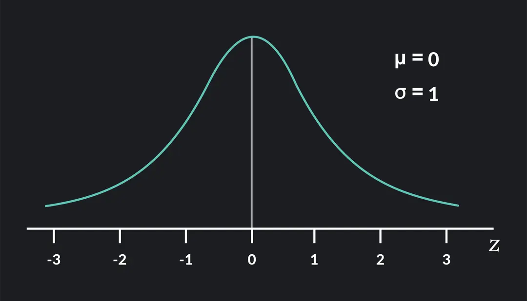
it is defined by equation
$$
[
q(z|x) = \mathcal{N}\big(\mu(x), \sigma^2(x)\big)
]
$$

When we sample like this the randomness and the network’s outputs are all mixed together in one step. Backpropagation cannot see clearly how changing ,So it cannot compute proper gradients.

To navigate thi issue we take
$$
[
\epsilon \sim \mathcal{N}(0,1)
]
$$
and
$$
[
z = \mu(x) + \sigma(x)\epsilon
]
$$
now all of the randomness is on ϵ and now, μ and σ are normal numbers, produced by the model.
In one line we can say ,Epsilon keeps the randomness separate from the learnable parameters, so the model stays random but still allows gradients to flow.

5. Implementaion¶

5.1. Model Definition¶

This model looks similar to a standard Autoencoder, having a symmetric encoder–decoder structure. However, in reality, it is very different from a standard AE.

We used a 5-layer structure:

Input → Hidden → Latent → Hidden → Output

The hidden layers in between are used to sequentially change the dimensionality rather than drastically change the dimensions in one step

The model uses a ReLU activation function between the hidden and latent layers, and a sigmoid activation function at the output layer.

ReLU is used to introduce nonlinearity, as discussed in the blog ("A Comparission between PCA and NLPCA").
Without nonlinearity, the model would behave like a linear transformation and would not be able to learn complex patterns in the data.

A sigmoid activation is used at the output because we are working with the MNIST dataset, which consists of grayscale images. Since pixel values are normalized between 0 and 1, using a sigmoid ensures that the output values also lie between 0 and 1. This helps the model produce valid reconstructions within the correct pixel range.

5.2 Training The Model¶

This is where we apply the ELBO and reparamterisation trick. First we must reduce the KL divergence to apply it to the model.

We know,
$$
[
D_{KL}(q(z|x)|p(z))
= \int q(z|x) \log \frac{q(z|x)}{p(z)} \, dz
]$$

Assume Gausian Distribution(Reparameterisation Trick)
$$
[
q(z|x) = \mathcal{N}(\mu, \sigma^2)
]$$
$$
[
D_{KL}(\mathcal{N}(\mu, \sigma^2) | \mathcal{N}(0,1))
=
\frac{1}{2}
\left(
\mu^2 + \sigma^2 - \log \sigma^2 - 1
\right)
]$$
$$
[
D_{KL}(q(z|x)|p(z))
=
\frac{1}{2}
\sum_{i=1}^{d}
\left(
\mu_i^2 + \sigma_i^2 - \log \sigma_i^2 - 1
\right)
]$$

We use this reduced form for training the model. However in practical model application,we come across a major issue

Up until now, everything sounds perfectly balanced.The reconstruction term pushes the model to reconstruct the input well.The KL term pushes the latent distribution to stay close to a simple prior.

But in practice, this balance is fragile. When training a VAE, two major problems can occur:

• KL Explosion
• Posterior collapse

KL Explosion¶

KL explosion happens when the

$$
[
D_{KL}(q(z|x)|p(z))
=
\frac{1}{2}
\sum_{i=1}^{d}
\left(
\mu_i^2 + \sigma_i^2 - \log \sigma_i^2 - 1
\right)
]$$

becomes very large during training. This happens due to the model's tendency to increase or decrese the value of μ or σ drastically .

looking at the σ part:
If σ² becomes very large → the σ² term dominates → KL grows large.
If σ² becomes very small → −log(σ²) becomes large → KL also grows large.

So both extremely large variance and extremely tiny variance increase KL.Why would σ grow large? Sometimes the encoder increases variance to reduce reconstruction pressure or because of unstable gradients early in training.

Why would σ shrink toward zero? To make the encoding almost deterministic and improve reconstruction.

Both extremes increase KL sharply

When either case happens:

• The loss becomes dominated by KL
• Gradients explode
• Training becomes unstable
• The model struggles because it is being strongly punished for deviating from the prior.

Posterior Collapse¶

This is the opposite scenario compared to KL explosion. It happens when,

q(z∣x)≈p(z).

This occurs because of how the KL divergence is perceived by the model. The objective tries to minimize the KL term. The easiest way to do this is by making q(z∣x)≈p(z), so that the KL divergence approaches zero.

In theory, this sounds perfect. However, what actually happens is that the encoder completely stops encoding meaningful information into z. The encoder was supposed to encode information from x into z, but now they become independent of each other. This pushes the model to ignore the encoder entirely, especially if the decoder is strong enough.

As a result, the decoder reconstructs data without relying on meaningful latent representations. The latent space becomes random noise with no structured relationship to the input.

5.3 The Beta Fix¶

We introduce a term ,β and multiply it with the KL Divergence term in the ELBO.

For KL Explosion,
When KL divergence becomes very large, we take a value β>1.

This gives more emphasis to the KL term. Since the KL term is subtracted in the objective, increasing β increases the penalty for large KL values. As a result, the model is pushed more strongly to reduce the KL divergence.

This prevents the KL term from growing uncontrollably, because the model is now actively penalized for letting it become too large.

For Posterior Collapse,
When posterior collapse happens, KL divergence becomes very small, often close to zero In this case, we take β<1.

This reduces the pressure on the KL term. The model is no longer strongly forced to minimize KL. As a result, the encoder is allowed to let q(z∣x) differ from p(z), which increases KL slightly and restores meaningful latent representations.

6. Outcomes¶

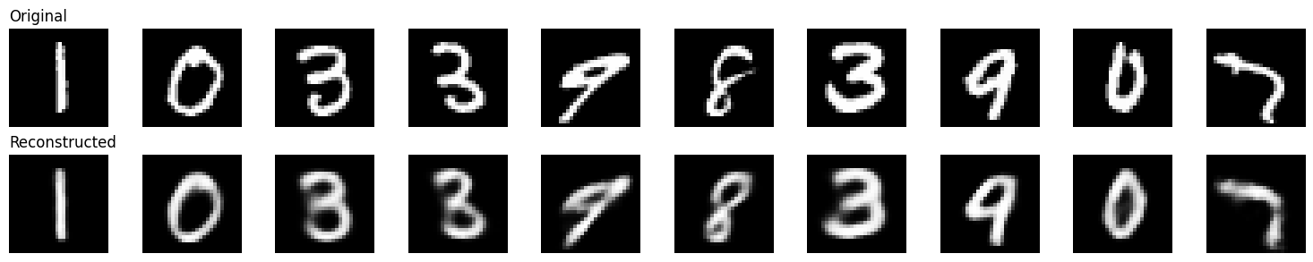
This is the reconstruction we get after implementing the model. As you can say we were fairly succesfull at recreating the MNIST data set however the results dont just end here.

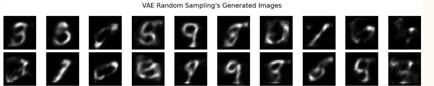
The above picture shows the strength of VAEs. This is an output after feeding random data directly into the latent space. This means we are directly bypassing the encoder layers completely.

Even if its not clear we can make out number-like features in these images. This is because of how VAE learn,their probabilistic nature helps them learn in such a way that it can also act not only as an autoencoder,but also as a generator.