My interest in science and astrophysics, combined with a growing fascination for machine learning, led me to explore a model that brings the best of both worlds together. In this blog, I’ll share what I’ve learned and walk you through how machine learning is now being used to make scientific tasks faster, smarter, and more efficient.

LIGO¶

LIGO is the Laser Interferometer Gravitational-Wave Observatory. It’s an observatory that doesn’t look at light, stars, or planets the way a normal telescope does. Instead, it listens to the universe.

Have you ever read an article about a newly discovered black hole where scientists somehow know how massive it is or how big it might be? It almost feels like guesswork, right? But it isn’t.

What LIGO detects are gravitational waves, tiny ripples in spacetime caused by massive events like black holes colliding. When two huge objects interact, they disturb spacetime itself, and that disturbance travels all the way to Earth.

Think of it like this: if you drop a rock into still water, waves spread out from the point of impact. Now imagine spacetime behaving like that water. Those ripples are what LIGO is designed to detect.

So how does LIGO actually measure and store this data?¶

At its core, LIGO uses lasers. It has two long arms placed perpendicular to each other. A laser beam is split into two, sent down both arms, reflected by mirrors, and brought back together.

Now here’s the cool part. When a gravitational wave passes through, it slightly stretches one arm and compresses the other. The change is insanely small, smaller than the width of a proton. For reference, a proton is about 1.7 × 10⁻¹⁵ meters small! But that tiny difference changes how the laser beams recombine.

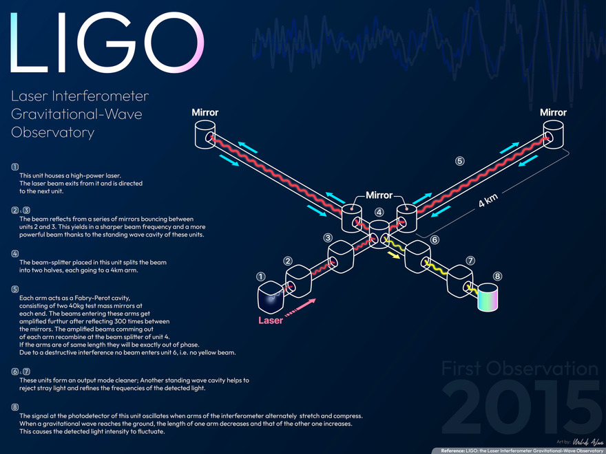
That change is recorded as data. LIGO is constantly collecting this data as a continuous stream over time. But here’s the problem, most of what it records is noise. Vibrations from the Earth, thermal effects, even distant human activity all get mixed in. The actual signal we care about is buried deep inside all that.

What Came Before: Match Filtering¶

So how do we find a real signal in all that noise? This is where match filtering comes in. Match Filtering is mainly a bunch of complicated math but to explain what is actually does, let us use an example.

Imagine you’re in a crowded room and a song is playing faintly in the background. If you already know the song, your brain can pick it out from the noise, regardless of all the other sounds in the room. You recognize the instruments used, beats it contains and the rhythm it follows.

Match filtering works in a similar way. Scientists generate thousands of possible templates, basically predictions of what a gravitational wave should look like for different kinds of events. Then LIGO’s data is scanned against all of these templates.

If something matches closely, there’s a good chance we’ve detected a real event.

But recently… we’ve started doing something even better¶

Instead of manually comparing data to templates, what if a system could just learn what a signal looks like?

A newer approach called deep filtering uses machine learning models, especially neural networks, to automatically detect and analyze signals. Instead of relying only on predefined templates, these models are trained on huge amounts of simulated data. Over time, they learn to recognize patterns autonomously.

That means they can:
- Detect signals faster
- Work better in noisy conditions
- Extract features like mass and spin automatically

In a way, instead of telling the system what to look for, we’re letting it figure things out by itself, and that’s what makes deep filtering so powerful.

What’s happening under the hood?¶

Deep filtering essentially uses a stack of two 1D convolutional neural networks (CNNs) to process gravitational wave data. Since LIGO data is a signal over time, not an image, we use a 1D CNN instead of the usual 2D one.

Think of the data as a long waveform. Now imagine a small window, called a kernel, sliding across that waveform. At each step, it looks at a small chunk of the data, learns patterns from it, and moves forward.

Instead of trying to understand everything at once, the network breaks the problem into small parts, learns local features, and then combines them into a bigger understanding. Over time, it starts recognizing things like oscillations, spikes, and full waveform patterns that indicate real events.

Why two networks?¶

Deep filtering uses two separate CNNs, each with a specific job.

1. The Detector
The first network answers a simple question, "is there a signal here or not?" It scans incoming data and separates noise from potential gravitational wave signals. This step needs to be fast and reliable.

2. The Predictor
Once a signal is detected, the second network takes over. Instead of just saying something is there, it tries to figure out what exactly happened. It extracts key features like the masses and other properties of the objects involved.

Putting it together¶

So instead of manually comparing data to thousands of templates, deep filtering creates a pipeline:

• First, detect whether something interesting exists
• Then, immediately analyze and extract meaningful information

All of this can happen much faster, often in real time. It’s like having one system constantly listening for anything unusual, and another that instantly understands and explains what just happened.

How do these networks actually learn?¶

Now comes the most interesting part: training.

At a high level, training is just a loop of:
see data → make a guess → measure error → improve

Step 1: Give it data (with answers)¶

You train these networks using simulated gravitational wave signals mixed with noise.
So the network sees:
- Pure noise
- Noise with signals
And for the predictor network, it also sees the correct physical parameters.

Step 2: The network makes a guess¶

The data passes through all the layers.
At the beginning, everything is random, so the predictions are not great.

• The detector guesses signal or no signal
• The predictor guesses properties like mass

Step 3: Measure how wrong it is¶

The output is compared with the correct answer.
This difference is called the loss. The bigger the loss, the worse the prediction.

Step 4: Adjust the network¶

This is where learning happens. The network goes backward through its layers and adjusts each kernel slightly to reduce the error. If a pattern was missed, it learns to detect it. If it reacted to noise, it learns to ignore it.

Step 5: Repeat¶

This process is repeated thousands of times.
Over time:
- Early layers learn simple patterns
- Deeper layers learn complex waveform structures

Training the two networks¶

The two CNNs are usually trained separately:

• The detector learns to identify whether a signal exists
• The predictor learns to estimate the properties of the signal

Even though we talk about layers, you don’t train them one by one. The entire network learns together, automatically figuring out what each layer should focus on.

Where Deep Filtering Falls Short¶

Now that we understand how deep filtering works, it’s important to realize that it isn’t perfect. Like any model, it comes with its own set of limitations.

Some key limitations¶

• It struggles with signals that differ from what it has seen during training
• Performance can degrade in highly noisy or unexpected conditions
• It mainly focuses on local patterns, which can limit its ability to capture long-range dependencies
• Scaling to more complex signal structures can become computationally expensive

A Direction I’ve Been Exploring¶

These limitations got me thinking. What if instead of relying purely on CNNs to process raw signals, we changed how the data is represented before it’s analyzed? I’m currently exploring a model architecture that tries to combine representation learning with sequence modeling.

Core Idea¶

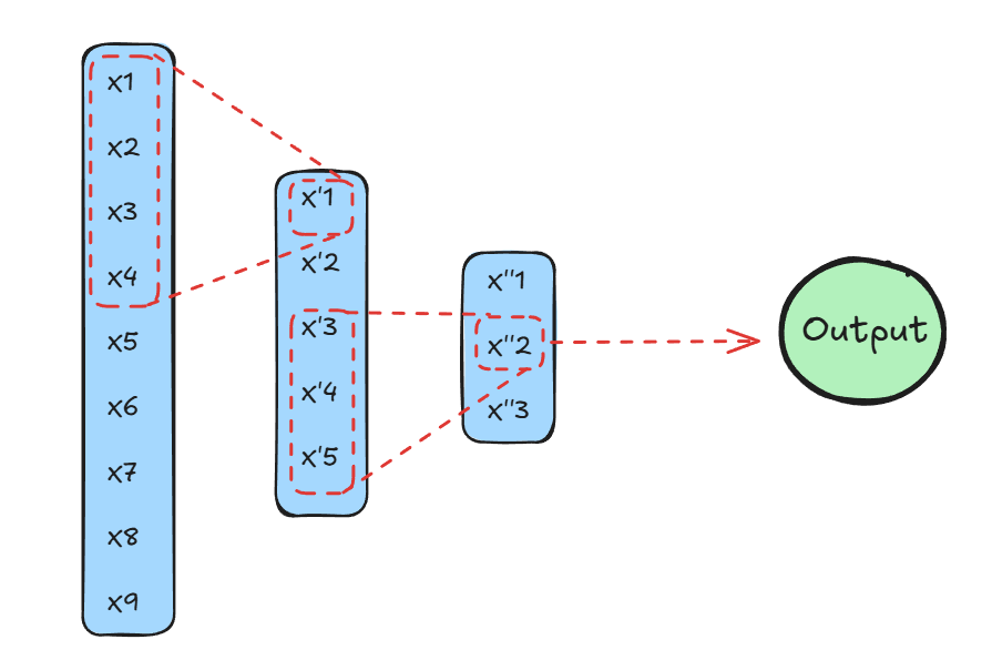
The idea is to first discretize the signal using an encoder.

• The encoder compresses the raw signal into a latent representation
• This latent space is then tokenized, turning it into a sequence of discrete elements

Once we have this sequence, it can be passed into a transformer model.

Why This Might Help¶

CNNs are very good at extracting local features, but they don’t naturally capture relationships across an entire signal. Transformers, on the other hand, are designed to model global dependencies.

So the intuition is:
- The encoder learns a compact and meaningful representation
- The tokenization step structures the data
- The transformer learns relationships across the full sequence

A Note on This Approach¶

This is still an idea I’m exploring, not a fully validated improvement over existing methods. The goal here is not to replace deep filtering outright, but to experiment with ways to make models:

• More adaptable
• Better at handling complex signals
• More robust to noise

In the next section, I’ll try to break down this architecture further and explore how it could actually be implemented.

A Quick Intuition for Transformers¶

Since this idea relies on transformers, it’s worth building a bit of intuition for how they work. At a high level, a transformer is a model designed to understand relationships within a sequence. This sequence could be words in a sentence, or in our case, tokens representing parts of a signal.

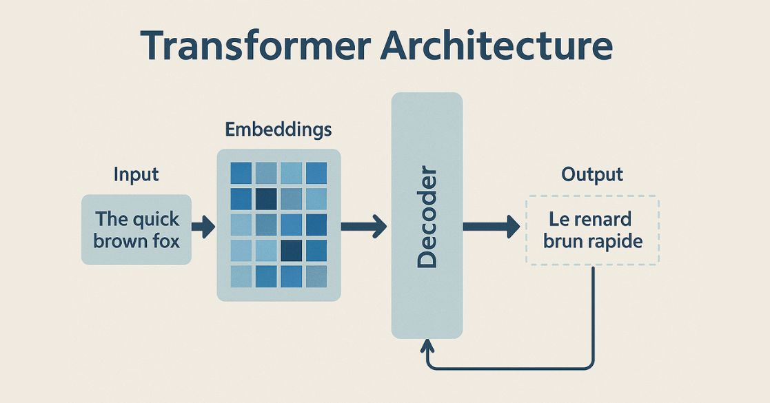
(Transformers are most commonly used in natural language processing, but in this case, we apply the same idea to time-series signals.)

How is it different from CNNs?¶

CNNs look at small chunks of data at a time. They slide a window across the input and focus on local patterns. Transformers do something very different. Instead of looking at just nearby values, a transformer can look at the entire sequence at once and learn how every part relates to every other part.

The core concept behind transformers is something called attention. You can think of attention as a way for the model to decide:

“Which parts of this input are important when understanding this specific part?”

For example:
- In a sentence, a word might depend on another word far away
- In a signal, one part of a waveform might relate to something that happened much earlier
Attention allows the model to connect these distant pieces directly.

What does the transformer actually do?¶

Once you feed in a sequence of tokens, the transformer:

1. Looks at all tokens together
2. Assigns importance (attention) between them
3. Builds a richer representation by combining this information

This process is repeated across multiple layers, allowing the model to learn increasingly complex relationships.

Why this fits our model¶

In our case:
- The encoder converts the signal into tokens
- The transformer processes those tokens

This means the model is no longer limited to local patterns. It can:
- Capture long-range dependencies
- Understand the overall structure of the signal
- Potentially detect patterns that CNNs might miss

If CNNs are like scanning a signal piece by piece,
transformers are like stepping back and looking at the entire signal at once, understanding how everything connects.

A natural question here is whether transformers are even the right choice.¶

They are built around attention and learning relationships within a sequence, but in signal data there is no strict guarantee that one part of the signal is related to another.
Unlike language, where structure is explicit, signals can often appear noisy or loosely connected.

However, transformers are still useful not because they assume relationships, but because they can learn when and where they exist. Instead of forcing connections, they dynamically focus on important regions across the entire signal.

This allows them to capture long-range patterns, ignore irrelevant noise, and adapt to complex structures when they appear.So the advantage here is not just modeling relationships, but giving the model the flexibility to decide what actually matters.

Putting It All Together: A Hybrid Architecture¶

Now that we have a basic idea of what the model architecture looks like, let’s link everything together into a single pipeline.
The goal here is to combine:
- Discretization (VQ-VAE-2)
- Anomaly detection (via reconstruction loss)
- Sequence modeling (transformers)

Step 1: Learning the Structure of Noise (VQ-VAE-2)¶

We start with VQ-VAE-2, a variant of a Vector Quantized Autoencoder where discretization is applied to the latent space Unlike a standard autoencoder, this model:
- Compresses the input signal
- Maps it to a discrete codebook (set of learned vectors)
- Reconstructs the signal from these discrete representations

The key idea here is how we train it. Instead of training on signals, the encoder is trained primarily on simulated noise (similar to what LIGO observes). Over time, it becomes very good at learning:

“What does normal noise look like?”

Step 2: Using Reconstruction Loss as a Signal¶

Once trained, we pass real data through this model.
- If the input is just noise → it reconstructs well
- If the input contains a real signal → reconstruction becomes worse

This difference shows up as reconstruction loss. So instead of directly detecting signals, the model is acting as a kind of anomaly detector, highlighting parts of the data that don’t fit the learned noise distribution.

Step 3: Discretizing the Signal¶

Because we’re using VQ-VAE-2:
- The latent space is not continuous
- Each part of the signal is mapped to a codebook index

This effectively converts the signal into a sequence of discrete tokens. At this stage, we now have two things:
- A tokenized representation of the signal
- A reconstruction loss map showing which regions are unusual

Step 4: Selecting What to Pass Forward¶

Instead of blindly feeding the entire latent space into the transformer, we use the reconstruction loss to guide us.
Rather than hard filtering, we use a soft selection approach:
- Regions with higher reconstruction loss are treated as more important
- We can select top-k segments or assign higher weights to these regions

This way:
- We prioritize likely signal regions
- But still retain enough context to avoid losing important information

Step 5: Transformer for Global Understanding¶

The selected (and structured) token sequence is then passed into a transformer.
Here, the model:
- Looks at the entire sequence
- Learns relationships between different regions
- Captures long-range dependencies in the signal

This allows it to move beyond local feature detection and understand the signal at a global level.

The Full Pipeline¶

You can think of the system in stages:
1. Learn noise → build a vocabulary of normal patterns
2. Spot deviations → use reconstruction loss to highlight anomalies
3. Discretize → convert the signal into tokens
4. Prioritize → focus on important regions without discarding context
5. Interpret → use a transformer to analyze the full structure

Instead of directly searching for signals in noisy data, this approach:
- Learns what “normal” looks like first
- Uses that to guide attention toward unusual regions
- Represents the data in a structured, tokenized form
- Applies global reasoning through a transformer

Important Note¶

This model does not strictly separate noise and signal.

Instead, it creates a structured way to highlight and analyze deviations from noise.

The effectiveness of this approach depends heavily on:
- How well the noise is modeled
- How the reconstruction loss threshold is tuned
- How much information is retained before the transformer

This is still an experimental idea, but it provides a framework for combining representation learning, anomaly detection, and sequence modeling into a single pipeline.¶